Basic R graphics for mapping
Dataframes of coordinates to make maps. There is a sample data file. Download the file and save it in your working directory. The first command here, setwd, tells R to use the designated directory. On my computer, the file is in ~/meetings_workshops/Rgis/data, but that will be different for everybody.
setwd('~/meetings_workshops/Rgis/data')
pan=read.delim('PanamaXY.csv')
Check the first few rows to understand what is in the file. They are x-y coordinates as longitude and latitude.
head(pan)
| X | Y | |
|---|---|---|
| 1 | -79.46 | 9.57 |
| 2 | -79.25 | 9.54 |
| 3 | -79.16 | 9.54 |
| 4 | -79.08 | 9.54 |
| 5 | -79.05 | 9.55 |
| 6 | -79.04 | 9.55 |
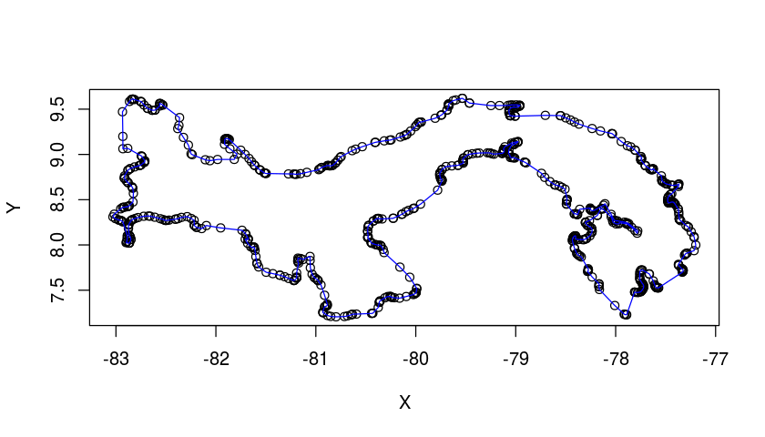
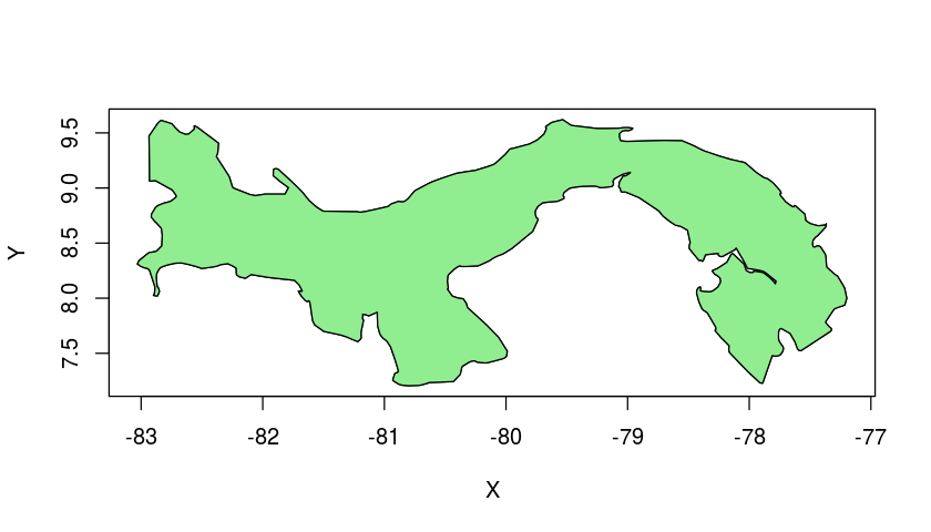
R's basic graphing functions work fine for making maps once coordinates are available. There is also a polygon function to fill areas.
plot(Y~X,data=pan)
lines(Y~X,data=pan,col='blue')
plot(Y~X,data=pan,type='l')
polygon(pan,col='lightgreen')
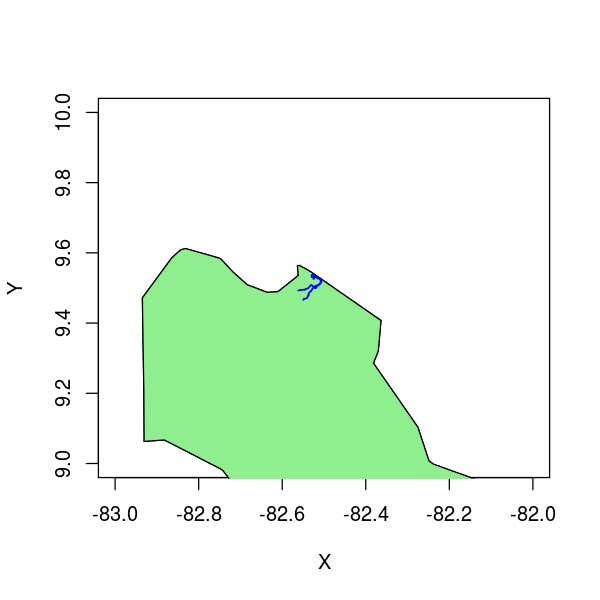
There are 8 files with San San River coordinates. Here are tricks with loops for quickly reading in the 8 files then combining them into one, using R's assign function to create variable names for all 8, and R's get function to open a variable by name. The combined file, named SS here, has extra rows of NAs between each section. This allows R to draw the map easily. [These use the function pst which is in the CTFS R Package. It's a revision of R's paste function that has no blank spaces. (Without the CTFS R Package, you have to use paste and set sep='' in the code below.) By inserting a row of NAs -- c(NA,NA,NA) -- between every section of the river, R will be able to draw the lines correctly. Without the row of NAs, R will draw connections from one line to the next.
setwd('~/meetings_workshops/Rgis/data')
for(j in 1:8) assign(pst('SanSanRiver',j),read.delim(pst('SanSanRiver',j,'.csv')))
head(SanSanRiver1)
      ID latitude longitude
1 1501.5 9.525676 -82.52445
2 1502.0 9.526057 -82.52483
3 1503.0 9.526057 -82.52509
4 1504.0 9.526861 -82.52509
5 1505.0 9.527221 -82.52524
6 1506.0 9.527623 -82.52507
head(SanSanRiver8)
    ID latitude longitude
1 80.5 9.505233 -82.51709
2 81.0 9.504090 -82.51737
3 82.0 9.502588 -82.51754
4 83.0 9.501530 -82.51775
5 84.0 9.500599 -82.51833
6 85.0 9.499244 -82.51919
SS=SanSanRiver1
for(j in 1:8) SS=rbind(SS,c(NA,NA,NA),get(pst('SanSanRiver',j)))
dim(SS)
[1] 1730 3
summary(SS)
       ID            latitude       longitude
 Min.   :   5.0   Min.   :9.466   Min.   :-82.56
 1st Qu.: 432.2   1st Qu.:9.482   1st Qu.:-82.55
 Median : 861.5   Median :9.495   Median :-82.54
 Mean   : 890.3   Mean   :9.500   Mean   :-82.54
 3rd Qu.:1381.8   3rd Qu.:9.519   3rd Qu.:-82.53
 Max.   :1655.0   Max.   :9.539   Max.   :-82.51
 NA's   :8        NA's   :8       NA's   :8
plot(Y~X,data=pan,type='l',xlim=c(-83,-82),ylim=c(9,10))
polygon(pan,col='lightgreen')
lines(latitude~longitude,data=SS,col='blue')
R GIS
Shape files
Shape files use a format designed for Arc Info (ESRI) whose sole purpose is to store and manage geographic data. They hold coordinates, just like R data.frames, but more information as well. Coordinates are organized into polygons (or lines), and additional data about those features can be included. We start with a sample shape database called TM_WORLD_BORDERS-0.3. There are four different files which you need, all with the same name but four different extensions (you don't need the readme file). R will treat them as one. Download all four into the same folder; you can save them anywhere, then use setwd to the folder. My copy of TM_WORLD_BORDERS-0.3 is in ~/data/gis/World.
You need sp and maptools packages to read these shape files. Then the function readShapePoly (package maptools) simply reads the shape file, using the main name. Save it to an R object, here named WorldGIS.
setwd('~/data/gis/World')
library(sp)
library(maptools)
worldGIS=readShapePoly('TM_WORLD_BORDERS-0.3')
class(worldGIS)
[1] "SpatialPolygonsDataFrame"
attr(,"package")
[1] "sp"
The resulting object, worldGIS, is a spatial data type called SpatialPolygonsDataFrame. This is a very complicated data type, difficult to understand in detail. It has map coordinates for 246 countries, and each country has multiple polygons. These spatial objects are advanced classes in R, built with slots and lists.
There are five slots in worldGIS. The bbox is small but useful -- the range of x and y coordinates. The data slot is a simple data.frame of 246 countries, with names and other information. Notice that slots within a class are accessed with the symbol @.
slotNames(worldGIS)
[1] "data" "polygons" "plotOrder" "bbox" "proj4string"
head(worldGIS@data)
  FIPS ISO2 ISO3 UN                NAME   AREA  POP2005 REGION SUBREGION     LON     LAT
0   AC   AG  ATG 28 Antigua and Barbuda     44    83039     19        29 -61.783  17.078
1   AG   DZ  DZA 12             Algeria 238174 32854159      2        15   2.632  28.163
2   AJ   AZ  AZE 31          Azerbaijan   8260  8352021    142       145  47.395  40.430
3   AL   AL  ALB  8             Albania   2740  3153731    150        39  20.068  41.143
4   AM   AM  ARM 51             Armenia   2820  3017661    142       145  44.563  40.534
5   AO   AO  AGO 24              Angola 124670 16095214      2        17  17.544 -12.296
worldGIS@bbox
   min      max
x -180 180.0000
y  -90  83.6236
The slot called polygons is a list, and it has a length. There are 246, one for each country. Each belongs to another class of spatial object called Polygons.
length(worldGIS@polygons)
[1] 246
class(worldGIS@polygons[[1]])
[1] "Polygons"
attr(,"package")
[1] "sp"
str(worldGIS@polygons[[1]])
Formal class 'Polygons' [package "sp"] with 5 slots
  ..@ Polygons :List of 2
  .. ..$ :Formal class 'Polygon' [package "sp"] with 5 slots
  .. .. .. ..@ labpt  : num [1:2] -61.8 17.1
  .. .. .. ..@ area   : num 0.0291
  .. .. .. ..@ hole   : logi FALSE
  .. .. .. ..@ ringDir: int 1
  .. .. .. ..@ coords : num [1:23, 1:2] -61.7 -61.7 -61.8 -61.9 -61.9 ...
  .. ..$ :Formal class 'Polygon' [package "sp"] with 5 slots
  .. .. .. ..@ labpt  : num [1:2] -61.8 17.6
  .. .. .. ..@ area   : num 0.0171
  .. .. .. ..@ hole   : logi FALSE
  .. .. .. ..@ ringDir: int 1
  .. .. .. ..@ coords : num [1:25, 1:2] -61.7 -61.7 -61.7 -61.7 -61.8 ...
  ..@ plotOrder: int [1:2] 1 2
  ..@ labpt    : num [1:2] -61.8 17.1
  ..@ ID       : chr "0"
  ..@ area     : num 0.0462
slotNames(worldGIS@polygons[[1]])
[1] "Polygons" "plotOrder" "labpt" "ID" "area"
One of those Polygons (capital-P) is yet another list. This first, for country 1, is a list of two. So the map of Antigua and Barbuda has two objects called Polygon, and each of those really is a polygon, with coordinates defining the boundary.
length(worldGIS@polygons[[1]]@Polygons)
[1] 2
str(worldGIS@polygons[[1]]@Polygons)
List of 2
 $ :Formal class 'Polygon' [package "sp"] with 5 slots
  .. ..@ labpt  : num [1:2] -61.8 17.1
  .. ..@ area   : num 0.0291
  .. ..@ hole   : logi FALSE
  .. ..@ ringDir: int 1
  .. ..@ coords : num [1:23, 1:2] -61.7 -61.7 -61.8 -61.9 -61.9 ...
 $ :Formal class 'Polygon' [package "sp"] with 5 slots
  .. ..@ labpt  : num [1:2] -61.8 17.6
  .. ..@ area   : num 0.0171
  .. ..@ hole   : logi FALSE
  .. ..@ ringDir: int 1
  .. ..@ coords : num [1:25, 1:2] -61.7 -61.7 -61.7 -61.7 -61.8 ...
head(worldGIS@polygons[[1]]@Polygons[[1]]@coords)
          [,1]     [,2]
[1,] -61.68667 17.02444
[2,] -61.73806 16.98972
[3,] -61.82917 16.99694
[4,] -61.87611 17.01694
[5,] -61.88056 17.01972
[6,] -61.88361 17.02361
Determine that Panama is row 165 in worldGIS@data. Panama has 17 Polygons. The last, number 17, is the biggest.
which(worldGIS@data$NAME=='Panama')
[1] 165
length(worldGIS@polygons[[165]]@Polygons)
[1] 17
dim(worldGIS@polygons[[165]]@Polygons[[17]]@coords)
[1] 716 2
Keeping track of the detailed structure of the SpatialPolygonsDataFrame is tedious, but fortunately the basic mapping tools do not require knowing the details. Simply use plot and subset to come up with basic graphs.
plot(worldGIS)

plot(subset(worldGIS,NAME=='Panama'))

CA=subset(worldGIS,NAME=='Panama' | NAME=='Costa Rica' | NAME=='Nicaragua' | NAME=='Honduras' | NAME=='Guatemala')
plot(CA)

bbox(CA)
         min       max
x -92.246780 -77.19833
y   7.206111  17.82111
CA@bbox
         min       max
x -92.246780 -77.19833
y   7.206111  17.82111
CA@data
    FIPS ISO2 ISO3  UN       NAME  AREA  POP2005 REGION SUBREGION     LON    LAT
38    CS   CR  CRI 188 Costa Rica  5106  4327228     19        13 -83.946  9.971
74    GT   GT  GTM 320  Guatemala 10843 12709564     19        13 -90.398 15.256
78    HO   HN  HND 340   Honduras 11189   683411     19        13 -86.863 14.819
158   NU   NI  NIC 558  Nicaragua 12140  5462539     19        13 -85.034 12.840
164   PM   PA  PAN 591     Panama  7443  3231502     19        13 -80.920  8.384
One way to understand the SpatialPolgonsDataFrame is to build one a step at a time from the bottom. There are functions in the sp package for creating each of the four spatial objects needed. Here I start with four sample data.frames available at the Sample Data page. There were saved as an rdata object, and I use the R function load for getting it. There are NOT ascii text, so read.delim will not work.
setwd('~/meetings_workshops/Rgis/data')
load('samplePoly.rdata')
ls(2)
head(pan1)
str(pan1)
Each of the four objects is a simple data.frame of coordinates, just like the ones we used for simple maps at the start of the workshop. There are two columns of x-y coordinates, and nothing else. The function Polygon converts them into a special GIS Class called Polygon.
The Polygon class has slots to store coordinates, the bbox, and the area, which it just calculated.pan1poly=Polygon(pan1) pan2poly=Polygon(pan2) us1poly=Polygon(us1) us2poly=Polygon(us2) class(pan1poly)
[1] "Polygon"
attr(,"package")
[1] "sp"
slotNames(pan1poly)
[1] "labpt" "area" "hole" "ringDir" "coords"
pan1poly@area
[1] 0.00163715
pan1poly@coords
              X        Y
 [1,] -81.77862 7.276388
 [2,] -81.79445 7.225555
 [3,] -81.79750 7.225833
 [4,] -81.80112 7.229444
 [5,] -81.80556 7.238610
 [6,] -81.81862 7.270000
 [7,] -81.81917 7.272499
 [8,] -81.81917 7.286944
 [9,] -81.81862 7.290000
[10,] -81.81612 7.291111
[11,] -81.81361 7.291111
[12,] -81.78778 7.285277
[13,] -81.77862 7.276388
attr(,"projection")
[1] "LL"
The two polygons called pan are part of the Panama map, so it now makes sense to combine them into a bigger object. The Class called Polygons does this. Likewise, the two polygons from the U.S. should be combined. Each becomes a list of two polygons.
panpolys=Polygons(list(pan1poly,pan2poly),ID='Panama')
uspolys=Polygons(list(us1poly,us2poly),ID='US')
class(panpolys)
[1] "Polygons"
attr(,"package")
[1] "sp"
length(panpolys@Polygons)
[1] 2
slotNames(panpolys@Polygons[[1]])
[1] "labpt" "area" "hole" "ringDir" "coords"
This is probably familiar now, since it is what the WorldGIS database built by readShapePoly looks like. There are two countries in this mini-database, each with two polygons. The next step is to join those two countries into a large object called a SpatialPolygon Class. Finally this produces an object which can be mapped with the plot function.
panus=SpatialPolygons(list(panpolys,uspolys))
class(panus)
[1] "SpatialPolygons"
attr(,"package")
[1] "sp"
slotNames(panus)
[1] "polygons" "plotOrder" "bbox" "proj4string"
plot(panus)

But it still lacking the data slot which the WorldGIS has. This comes in the next, and final, step, creating the SpatialPolygonDataFrame object. The data.frame must be constructed, and can include any columns. But there must be two rows, and those rows must have row.names matching the IDs assigned to the Polygons Classes. This is the same class as WorldGIS, and has all five slots.
datafile=data.frame(row.names=c('Panama','US'),continent=c('CA','NA'))
panusdf=SpatialPolygonsDataFrame(panus,datafile)
class(panusdf)
[1] "SpatialPolygonsDataFrame"
attr(,"package")
[1] "sp"
slotNames(panusdf)
[1] "data" "polygons" "plotOrder" "bbox" "proj4string"
Converting lat-long to UTM
UTM coordinates are another way of mapping locations, frequently used by GPS, in small-scale mapping. Units are in either meters or kilometers, making them convenient for understanding distances on a map. UTM coordinates should not be used for large areas (> 300 km).
The package PBSmapping has a function that easily converts between lat-long and UTM in a data.frame with coordinates. It is illustrated here with the pan1 data.frame just used in the sample above. Note that the function convUL requires that the data.frame have columns named X and Y and has an attribute named projection that has a value 'LL' or 'UTM'. The steps below convert pan1 to UTM then back to lat-long. Once pan1 is converted to UTM, it can be passed to the Polygon function to get the area in square kilometers.
head(pan1)
             X        Y
[1,] -81.77862 7.276388
[2,] -81.79445 7.225555
[3,] -81.79750 7.225833
[4,] -81.80112 7.229444
[5,] -81.80556 7.238610
[6,] -81.81862 7.270000
colnames(pan1)=c('X','Y')
attr(pan1,'projection')='LL'
pan1utm=convUL(pan1)
head(pan1utm)
         X        Y
1 414.0491 804.3768
2 412.2924 798.7598
3 411.9555 798.7911
4 411.5569 799.1910
5 411.0685 800.2053
6 409.6327 803.6783
Polygon(pan1utm)@area
[1] 19.98201
pan1LL=convUL(pan1utm)
Raster data
Functions in R base package for raster maps
Map data in raster format comes in a grid, covering x-y coordinates on a complete checkerboard pattern. At each set of coordinates, there is an 'attribute'. I created a mini sample dataset to illustrate how raster data look and to use the base functions R has for mapping raster data. It is a matrix with 5 rows and 10 columns, with each element a single hectare of the 50-ha plot at Barro Colorado. The value is the number of tree species that are > 30 cm in diameter. The matrix represents a map, with the top row referring to the south row of hectares of the plot, covering 10 ha and 1000 meters, and the left column referring to the west column of 5 hectares. In other words, the matrix is a representation of a plot map, but it's upside-down, with south above and north below. That's entirely arbitrary -- it's just how I built it. In order to show this matrix with north at the top, you can turn it upside down by requesting rows in backwards order.
setwd('~/meetings_workshops/Rgis/data')
load('~/meetings_workshops/Rgis/data/diversityBCI.rdata')
diversityBCI
     [,1] [,2] [,3] [,4] [,5] [,6] [,7] [,8] [,9] [,10]
[1,]   38   38   36   29   39   38   34   44   35    27
[2,]   29   32   33   38   31   32   27   29   38    34
[3,]   38   33   33   39   39   41   41   33   34    33
[4,]   32   37   38   34   27   36   45   34   29    32
[5,]   38   38   33   31   38   40   34   39   34    31
diversityBCI[5:1,]
     [,1] [,2] [,3] [,4] [,5] [,6] [,7] [,8] [,9] [,10]
[1,]   38   38   33   31   38   40   34   39   34    31
[2,]   32   37   38   34   27   36   45   34   29    32
[3,]   38   33   33   39   39   41   41   33   34    33
[4,]   29   32   33   38   31   32   27   29   38    34
[5,]   38   38   36   29   39   38   34   44   35    27
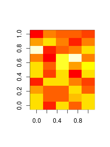
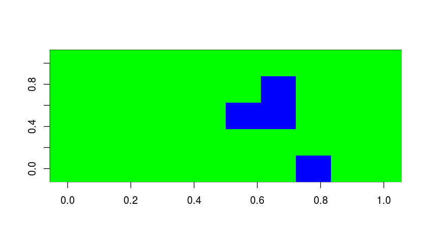
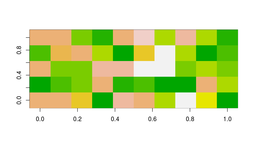
R has a function image to draw a map of any matrix. It works without any other information, but in this default format, notice that it rotates the map. Running the first command below produces a map with 5 columns and 10 rows. I would prefer a map that has north at the top, and this works with the function t, meaning the transpose of a matrix (that's from basic algebra, exchanging rows and columns. The second image, using diversityBCI has north at the top. This is curious, because the matrix has north at the bottom. It is useful for me to remember to display the matrix on the screen with rows inverted, diversityBCI[5:1,], and to use image with the transpose. Then the map and the matrix correspond exactly. The commands below show some options for colors; with images, you can assign any breaks you like, but there must always be one less color.
image(diversityBCI)
t(diversityBCI)
      [,1] [,2] [,3] [,4] [,5]
 [1,]   38   29   38   32   38
 [2,]   38   32   33   37   38
 [3,]   36   33   33   38   33
 [4,]   29   38   39   34   31
 [5,]   39   31   39   27   38
 [6,]   38   32   41   36   40
 [7,]   34   27   41   45   34
 [8,]   44   29   33   34   39
 [9,]   35   38   34   29   34
[10,]   27   34   33   32   31
image(t(diversityBCI),breaks=c(0,40,70),col=c('green','blue'))
image(t(diversityBCI),breaks=c(0,30:40,70),col=terrain.colors(12))
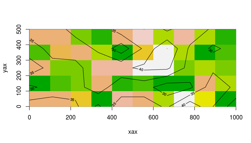
Notice that the matrix by itself carries no information about the coordinates. It's not a GIS object, just a bare matrix. You have to supply coordinates. This works by providing x and y values. The number of x values must match the number of columns on the map, and y the number of rows. The 50-ha plot runs from x=0 to x=1000 and y=0 to y=500. To get these coordinates correct, I need 10 numbers starting at 50 and ending at 950 (or 450 for y). This is because the grid cells are 100 m across, and the first column is thus centered at 50. The x and y values you provide are matched to the center of the grid cells. When this is done correctly, you can overlay points or lines and they will be at the right place. With this sort of plot map, I often overlay points for trees using the tree coordinates, as in the example below for a tree at x=122, y=356.
xax=seq(50,950,len=10)
yax=seq(50,450,len=5)
image(x=xax,y=yax,z=t(diversityBCI),breaks=c(0,30:40,70),col=heat.colors(12))
abline(h=250)
points(122,356)
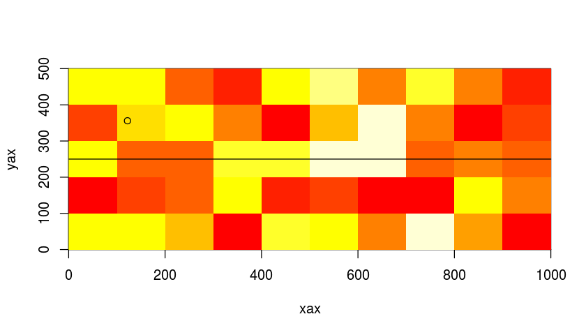
There are two other functions in the R base package that work similarly to image, both to draw contour lines. A confusing aspect, however, is getting contour and image maps to overlay correctly. The call
xaxc=seq(0,1000,len=10)
yaxc=seq(0,500,len=5)
image(x=xax,y=yax,z=t(diversityBCI),breaks=c(0,30:40,70),col=terrain.colors(12))
contour(x=xaxc,y=yaxc,z=t(diversityBCI),nlevels=5,add=TRUE)
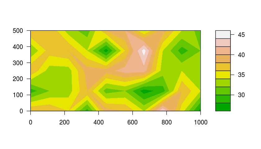
The function filled.contour has the great advantage of showing a legend. It has the great disadvantage, however, of not overlaying correctly: the legend takes up space on the map, and points will not appear in the right place. I have never solved this, and never overlay on filled contours. (R base does have a function legend which you can use to build your own legends on images, but I am not showing it here.
filled.contour(x=xaxc,y=yaxc,z=t(diversityBCI),nlevels=10,col=terrain.colors(10))
R GIS for raster data
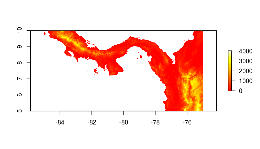
The package named raster has many tools for reading, manipulating, and mapping raster data. Just like the Spatial Classes for polygons, it works with Spatial Classes for raster, and these allow easy loading mapping without any understanding of what's inside. Below, the function raster creates a RasterLayer class using special geotiff files for world topography. These srtm elevation files (90-m topography for the entire world) are available online in chunks of 5x5 degrees. Panama happens to span two pieces, which is why I use two below, with the function merge to combine them. The data below are huge -- two files with 36 million points each -- and your computer may encounter slow downs trying to use it. In the commands below, I remove the first two objects after merging to reduce the strain on R's memory. Cropping the data to a smaller size is easy with raster, and the steps below move right there.
library(raster)
setwd('~/data')
rast21=raster('gis/elevationCRPan/srtm_21_11.tif')
rast20=raster('gis/elevationCRPan/srtm_20_11.tif')
class(rast21)
[1] "RasterLayer"
attr(,"package")
[1] "raster"
slotNames(rast21)
[1] "file" "data" "legend" "title" "extent" "rotated" "rotation" "ncols" "nrows" "crs" "history" "z"
str(rast21@extent)
Formal class 'Extent' [package "raster"] with 4 slots
  ..@ xmin: num -80
  ..@ xmax: num -75
  ..@ ymin: num 5
  ..@ ymax: num 10
rast21@extent
class       : Extent
xmin        : -80.00042
xmax        : -74.99958
ymin        : 4.999583
ymax        : 10.00042
rast21@nrows
[1] 6001
rast21@ncols
[1] 6001
total=merge(rast20,rast21)
rm(rast21)
rm(rast20)
total@extent
class       : Extent
xmin        : -85.00042
xmax        : -74.99958
ymin        : 4.999583
ymax        : 10.00042
class(total)
[1] "RasterLayer"
attr(,"package")
[1] "raster"
plot(total,col=heat.colors(20))
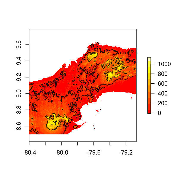
To crop, you need to create an Extent object, what raster calls a bounding box. There is a function called drawExtent() to create an extent by clicking on the map. Note that you must click on the map after executing! Nothing happens until you click.
ext=drawExtent()
You can also create an Extent object manually.
canalext=extent(-80.4,-79.07, 8.5, 9.7)
canal=crop(total,canalext)
plot(canal,col=heat.colors(10))
contour(canal,add=TRUE,levels=c(100,500,1000))
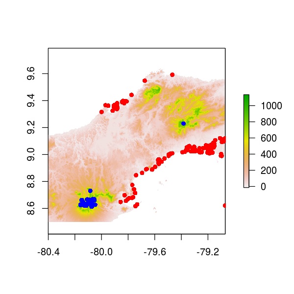
The package includes straightforward tools for getting at the data. This makes it possible to explore the data, for example to find the points where elev<0 (must be errors in the satellite data), or the highest points.
elev=getValues(canal)
length(elev)
[1] 2298240
summary(elev)
   Min. 1st Qu.  Median    Mean 3rd Qu.    Max.    NA's
  -26.0    49.0   123.0   181.7   250.0  1173.0 1010129
coord=xyFromCell(canal,cell=1:length(elev))
xyz=data.frame(coord,elev)
head(xyz)
          x        y elev
1 -80.40000 9.699167   NA
2 -80.39917 9.699167   NA
3 -80.39833 9.699167   NA
4 -80.39750 9.699167   NA
5 -80.39667 9.699167   NA
6 -80.39583 9.699167   NA
summary(xyz)
       x                y              elev
 Min.   :-80.40   Min.   :8.500   Min.   : -26.0
 1st Qu.:-80.07   1st Qu.:8.800   1st Qu.:  49.0
 Median :-79.74   Median :9.100   Median : 123.0
 Mean   :-79.74   Mean   :9.100   Mean   : 181.7
 3rd Qu.:-79.40   3rd Qu.:9.399   3rd Qu.: 250.0
 Max.   :-79.07   Max.   :9.699   Max.   :1173.0
                                  NA's   :1010129
plot(canal)
points(y~x,subset(xyz,elev<(-0)),col='red',pch=16)
points(y~x,data=subset(xyz,elev>1000),col='blue',pch=16)
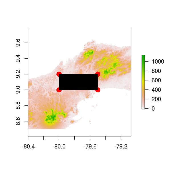
A useful function for raster data is point.in.polygon in the sp package. This example starts with a square polygon, creating a dataframe with four corners. Passing all the points from the raster and the one polygon produces a vector of one value per point, in this case __, equal to 1 if the point is inside, 0 if it's outside. A more useful example would be to use a polygon such as a national park; then you could explore elevation only within the park. The splancs package also has a function to test which points are inside a polygon: inout, inpip, pip.
samplepoly=data.frame(x=c(-80,-80,-79.5,-79.5),y=c(9,9.2,9.2,9))
samplepoly
      x   y
1 -80.0 9.0
2 -80.0 9.2
3 -79.5 9.2
4 -79.5 9.0
test=point.in.polygon(point.x=xyz$x,point.y=xyz$y,pol.x=samplepoly$x,pol.y=samplepoly$y)
table(test)
test
      0       1
2154240  144000
plot(canal)
points(y~x,samplepoly,col='red',pch=16,cex=2)
points(y~x,data=subset(xyz,test==1),pch=16,cex=.1)
